Build your own neural network using Machine Learning & TensorFlow

Welcome to the exciting world of machine learning! If you missed attending our workshop in-person, don’t worry; we’ve got you covered.
In this blog post, we’ll walk you through the key concepts and activities we covered during the workshop, all while keeping things both informative and, dare I say it, a bit funny.
Introduction: Unveiling the Power of Machine Learning
As software engineers, we’re no strangers to the art of coding. We break down complex problems into manageable pieces and write code to bring our ideas to life. Whether it’s creating stock analytics or designing a game, we’ve got the tools and skills to make it happen.
But machine learning, my friends, is a game-changer. It flips the script. Instead of us defining the rules, we let the computer figure them out. Imagine you want to recognize different activities like walking, running, or even golfing based on speed data. Traditionally, we’d write code to handle each case, but in the machine learning paradigm, we feed it lots of examples and let the computer work its magic.
Activity recognition example: Let the data speak
Take activity recognition, for instance. If you want to detect walking, running, biking, or even golfing based on speed, it’s not as simple as it sounds. People walk and run at varying speeds, uphill and downhill, and they do so differently from one another. The new approach? Gather loads of examples with labels—this is what walking looks like, this is running, this is biking, and yes, even this is golfing. Then, let the computer deduce the rules.
That’s the beauty of machine learning. It doesn’t just offer a fresh approach to problem-solving; it opens up new realms of possibilities that were once considered unfeasible.
What is a Neural Network?
Neural nets are a means of doing machine learning, in which a computer learns to perform some task by analyzing training examples. Usually, the examples have been hand-labeled in advance. An object recognition system, for instance, might be fed thousands of labeled images of cars, houses, coffee cups, and so on, and it would find visual patterns in the images that consistently correlate with particular labels.
These are the components of Neural Networks:
- Input — This is the data/values passed to the neurons
- Deep Neural Network (DNN) — This is an ANN with many hidden layers (layers between the input (first) layer and the output (last) layer)
- Weights — These values explain the strength (degree of importance) of the connection between any two neurons
- Bias — is a constant value added to the sum of the product between input values and respective weights. It is used to accelerate or delay the activation of a given node
- Activation function —calculates the output of the node (based on its inputs and the weights on individual inputs
Hello Neural Networks: The magic behind Machine Learning
Now, let’s dive into the basics of creating a neural network for pattern recognition. Don’t be intimidated; it’s not as complex as it may seem. In fact, it’s rather straightforward.
Imagine you have a set of numbers, and you need to find a pattern among them. Here’s a simple example:
Python

x = -1, 0, 1, 2, 3, 4

y = -3, -1, 1, 3, 5, 7
You probably figured that out quickly, right? You plugged in a few values for ‘x,’ saw that it fit the pattern, and voila! You’ve just done the basics of machine learning in your head.
Python

y = 2x - 1
We used Google Colaboratory for this workshop, a fantastic research tool for machine learning. It’s essentially a Jupyter notebook environment that requires zero setup and is entirely free to use. But don’t just take my word for it—let’s jump into the deep learning world.
We’ll be working with TensorFlow, a powerful library for machine learning, and its user-friendly API, Keras.
The simplicity of neural networks
Let’s start by creating a neural network. Don’t worry; it’s not as intimidating as it may sound. In Keras, we use the term “Dense” to define layers of connected neurons. A neural network can be as simple as a single neuron, and here’s how you create it:
Python

import numpy as np
from tensorflow import keras

# Define a layer with a single neuron
layer = keras.layers.Dense(units=1, input_shape=[1])

# Create a sequential model
model = keras.Sequential(layer)
The input shape here is super simple—just one value. You don’t need to be a math whiz for this; TensorFlow and Keras handle a lot of the heavy lifting when it comes to complex math.
Loss functions and optimizers: Behind the scenes
Now, let’s talk about the gears turning behind the scenes. When your neural network makes a guess (which is often random at first), it needs to learn from its mistakes and make better guesses. This is where loss functions and optimizers come into play.
Python

model.compile(optimizer='sgd', loss='mean_squared_error')
The loss function measures how good or bad a guess is. The optimizer uses this information to make the next guess even better. With each iteration, the guesses improve, and the accuracy approaches 100%. This process is known as convergence.
Let’s get practical
Enough theory; let’s get our hands dirty. We’ll start with a simple example: predicting the output of a function. Here’s the code:
Python

xs = np.array([-2.0, -1.0, 0.0, 1.0, 2.0, 3.0], dtype=float)
ys = np.array([-3.0, -1.0, 1.0, 3.0, 5.0, 7.0], dtype=float)

model.fit(xs, ys, epochs=500)

print(model.predict([10.0]))
You might expect the output to be 19, but it’s not quite that precise. But when you try this in the workbook yourself you will see it gives me a value close to 19 not 19. Why do you think this happens because the equation is y = 2x-1 ? There are two main reasons:
The first is that you trained it using very little data. There are only six points. Those six points are linear but there’s no guarantee that for every X, the relationship will be Y equals 2X minus 1. There’s a very high probability that Y equals 19 for X equals 10, but the neural network isn’t positive. So it will figure out a realistic value for Y. The second main reason. When using neural networks, as they try to figure out the answers for everything, they deal in probability. You’ll see that a lot and you’ll have to adjust how you handle answers to fit. Keep that in mind as you work through the code.
Building a house price predictor
Now that you’ve dipped your toes into the world of neural networks, it’s time to level up. We’re going to build a more complex model: a house price predictor. Here’s a sneak peek:
In this exercise you’ll try to build a neural network that predicts the price of a house according to a simple formula.
So, imagine if house pricing was as easy as a house costs 50k + 50k per bedroom, so that a 1 bedroom house costs 100k, a 2 bedroom house costs 150k etc.
How would you create a neural network that learns this relationship so that it would predict a 7 bedroom house as costing close to 400k etc.?
Hint: Your network might work better if you scale the house price down. You don’t have to give the answer 400…it might be better to create something that predicts the number 4, and then your answer is in the ‘hundreds of thousands’ etc.
Here is my solution – also available in the notebook:
Python

def house_model(y_new):
    xs=[]
    ys=[]
    for i in range(1,10):
        xs.append(i)
        ys.append((1+float(i))*50)

    xs=np.array(xs,dtype=float)
    ys=np.array(ys, dtype=float)
    layer = keras.layers.Dense(units = 1, input_shape = [1])
    model = keras.Sequential([layer])
    model.compile(optimizer='sgd', loss='mean_squared_error')

    model.fit(xs, ys, epochs = 4500)
    return (model.predict(y_new))
That was it, the basics. You even created a neural net all by yourself and made pretty accurate predictions too. Next, we will see about using some image classifiers with TensorFlow so stay tuned and explore till then.
Classify skin diseases with Deep Learning
Skin cancer is a significant health concern, but early detection can make a world of difference. In this section, we’ll delve into the world of deep learning and neural networks to create a skin disease classifier that can distinguish between benign and malignant skin conditions from photographic images.
Link to the Colab notebook: Workshop.ipynb
Key steps of solving this problem
Import the necessary modules, define some constants
Python

import os
import glob
import zipfile
import random

import tensorflow as tf
import tensorflow_hub as hub
import matplotlib.pyplot as plt
import numpy as np
import pandas as pd
from tensorflow.keras.utils import get_file


# to get consistent results after multiple runs
tf.random.set_seed(7)
np.random.seed(7)
random.seed(7)

tf.keras.backend.clear_session()

# 0 for benign, 1 for malignant
class_names = ["benign", "malignant"]

# training parameters
batch_size = 64
optimizer = "rmsprop"
loss = "binary_crossentropy"
A glimpse into the dataset
Before we jump into the coding, let’s understand our dataset. We’ll be using a portion of the ISIC archive dataset, which contains images of various skin diseases. Here’s how to get your hands on it:
Python

def download_and_extract_dataset():
  train_url = "https://ews0921.s3.eu-central-1.amazonaws.com/train.zip"
  valid_url = "https://ews0921.s3.eu-central-1.amazonaws.com/valid.zip"
  test_url  = "https://ews0921.s3.eu-central-1.amazonaws.com/test.zip"

  for i, download_link in enumerate([valid_url, train_url, test_url]):
    temp_file = f"temp{i}.zip"
    data_dir = get_file(origin=download_link, fname=os.path.join(os.getcwd(), temp_file))
    print("Extracting", download_link)
    with zipfile.ZipFile(data_dir, "r") as z:
      z.extractall("data")
    # remove the temp file
    os.remove(temp_file)

download_and_extract_dataset()
This dataset will be our playground for building a skin disease classifier.
Labeling the data
To train our model, we need labeled data. We’ll classify skin diseases into two categories: benign (nevus and seborrheic keratosis) and malignant (melanoma). We’ll generate metadata CSV files to label our data.
Python

# preparing data
# generate CSV metadata file to read img paths and labels from it
def generate_csv(folder, label2int):
    folder_name = os.path.basename(folder)
    labels = list(label2int)
    # generate CSV file
    df = pd.DataFrame(columns=["filepath", "label"])
    i = 0
    for label in labels:
        print("Reading", os.path.join(folder, label, "*"))
        for filepath in glob.glob(os.path.join(folder, label, "*")):
            df.loc[i] = [filepath, label2int[label]]
            i += 1
    output_file = f"{folder_name}.csv"
    print("Saving", output_file)
    df.to_csv(output_file)

# generate CSV files for all data portions, labeling nevus and seborrheic keratosis
# as 0 (benign), and melanoma as 1 (malignant)
generate_csv("data/train", {"nevus": 0, "seborrheic_keratosis": 0, "melanoma": 1})
generate_csv("data/valid", {"nevus": 0, "seborrheic_keratosis": 0, "melanoma": 1})
generate_csv("data/test", {"nevus": 0, "seborrheic_keratosis": 0, "melanoma": 1})
The generate_csv() function accepts 2 arguments, the first is the path of the set.
The second parameter is a dictionary that maps each skin disease category to its corresponding label value (again, 0 for benign and 1 for malignant).
The reason I did a function like this is the ability to use it on other skin disease classifications (such as melanocytic classification), so you can add more skin diseases and use it for other problems as well.
Now, our dataset is ready for action.
Loading and preparing the data
Loading and preparing the data is a crucial step in any machine learning project. We’ll load our data into DataFrames and preprocess the images.
Python

train_metadata_filename = "train.csv"
valid_metadata_filename = "valid.csv"

# load CSV files as DataFrames
df_train = pd.read_csv(train_metadata_filename)
df_valid = pd.read_csv(valid_metadata_filename)

n_training_samples = len(df_train)
n_validation_samples = len(df_valid)

print("Number of training samples:", n_training_samples)
print("Number of validation samples:", n_validation_samples)

train_ds = tf.data.Dataset.from_tensor_slices((df_train["filepath"], df_train["label"]))
valid_ds = tf.data.Dataset.from_tensor_slices((df_valid["filepath"], df_valid["label"]))
Decode the images
Python

# preprocess data
def decode_img(img):
  # convert the compressed string to a 3D uint8 tensor
  img = tf.image.decode_jpeg(img, channels=3)
  # Use `convert_image_dtype` to convert to floats in the [0,1] range.
  img = tf.image.convert_image_dtype(img, tf.float32)
  # resize the image to the desired size.
  return tf.image.resize(img, [299, 299])


def process_path(filepath, label):
  # load the raw data from the file as a string
  img = tf.io.read_file(filepath)
  img = decode_img(img)
  return img, label


valid_ds = valid_ds.map(process_path)
train_ds = train_ds.map(process_path)
Prepare the dataset for the training
def prepare_for_training(ds, cache=True, batch_size=64, shuffle_buffer_size=1000):
  if cache:
    if isinstance(cache, str):
      ds = ds.cache(cache)
    else:
      ds = ds.cache()
  # shuffle the dataset
  ds = ds.shuffle(buffer_size=shuffle_buffer_size)
  # Repeat forever
  ds = ds.repeat()
  # split to batches
  ds = ds.batch(batch_size)
  # `prefetch` lets the dataset fetch batches in the background while the model
  # is training.
  ds = ds.prefetch(buffer_size=tf.data.experimental.AUTOTUNE)
  return ds

valid_ds = prepare_for_training(valid_ds, batch_size=batch_size, cache="valid-cached-data")
train_ds = prepare_for_training(train_ds, batch_size=batch_size, cache="train-cached-data")
Here is what we did:
- cache(): Since we’re making too many calculations on each set, we used cache() method to save our preprocessed dataset into a local cache file, this will only preprocess it the very first time (in the first epoch during training).
- shuffle(): To basically shuffle the dataset, so the samples are in random order.
- repeat(): Every time we iterate over the dataset, it’ll keep generating samples for us repeatedly, this will help us during the training.
- batch(): We batch our dataset into 64 or 32 samples per training step.
- prefetch(): This will enable us to fetch batches in the background while the model is training.
Visualizing the data
A picture is worth a thousand words, and in our case, it might just save lives. Let’s visualize our dataset.
Python

batch = next(iter(valid_ds))

def show_batch(batch):
  plt.figure(figsize=(12,12))
  for n in range(25):
      ax = plt.subplot(5,5,n+1)
      plt.imshow(batch[0][n])
      plt.title(class_names[batch[1][n].numpy()].title())
      plt.axis('off')

show_batch(batch)
As you can see, distinguishing between malignant and benign skin diseases from images alone can be challenging. But that’s where our model comes in.
Building the model
Our skin disease classifier will be powered by a pre-trained InceptionV3 model, courtesy of TensorFlow Hub. Here’s how we assemble it:
Python

# building the model
# InceptionV3 model & pre-trained weights
module_url = "https://tfhub.dev/google/tf2-preview/inception_v3/feature_vector/4"

model = tf.keras.Sequential([
    hub.KerasLayer(module_url, output_shape=[2048], trainable=False),
    tf.keras.layers.Dense(1, activation="sigmoid")
])

model.build([None, 299, 299, 3])

model.compile(loss="binary_crossentropy", optimizer=optimizer, metrics=["accuracy"])

model.summary()
Notice before, we resized all images to (299, 299, 3), and that’s because of what InceptionV3 architecture expects as input, so we’ll be using transfer learning with TensorFlow Hub library to download and load the InceptionV3 architecture along with its ImageNet pre-trained weights.
We set trainable to False so we won’t be able to adjust the pre-trained weights during our training, we also added a final output layer with 1 unit that is expected to output a value between 0 and 1 (close to 0 means benign, and 1 for malignant).
After that, since this is a binary classification, we built our model using binary crossentropy loss, and used accuracy as our metric (not that reliable metric, we’ll see sooner why), here is the output of our model summary:
Training the model
Now comes the exciting part—training the model with our dataset.
Python

model_name = f"benign-vs-malignant_{batch_size}_{optimizer}"
modelcheckpoint = tf.keras.callbacks.ModelCheckpoint(model_name + "_{val_loss:.3f}.h5", save_best_only=True, verbose=1)

model.fit(train_ds,
                validation_data=valid_ds,
                steps_per_epoch=n_training_samples // batch_size,
                validation_steps=n_validation_samples // batch_size,
                verbose=1,
                epochs=25,
                callbacks=[modelcheckpoint]
)
We used ModelCheckpoint callback to save the best weights so far on each epoch, that’s why we set epochs to 100, that’s because it can converge to better weights at any time, to save your time, feel free to reduce that to 30 or so.
Since the fit() method doesn’t know the number of samples there are in the dataset, we need to specify steps_per_epoch and validation_steps parameters for the number of iterations (the number of samples divided by the batch size) of the training set and validation set respectively.
Now that we’ve trained our model to predict the benign and malignant classes, let’s make a function that predicts the class of any image passed to it.
Now let’s load our optimal weights that were saved by ModelCheckpoint during the training:
It says that the 0.44331 has the best weights so we need the following model:
You may not have the exact filename of the optimal weights, you need to search for the saved weights in the current directory that has the least loss.
Model evaluation with the test samples
Python

# evaluation
# load testing set
test_metadata_filename = "test.csv"

df_test = pd.read_csv(test_metadata_filename)

n_testing_samples = len(df_test)

print("Number of testing samples:", n_testing_samples)

test_ds = tf.data.Dataset.from_tensor_slices((df_test["filepath"], df_test["label"]))

def prepare_for_testing(ds, cache=True, shuffle_buffer_size=1000):
  if cache:
    if isinstance(cache, str):
      ds = ds.cache(cache)
    else:
      ds = ds.cache()
  ds = ds.shuffle(buffer_size=shuffle_buffer_size)
  return ds

test_ds = test_ds.map(process_path)

test_ds = prepare_for_testing(test_ds, cache="test-cached-data")

# convert testing set to numpy array to fit in memory (don't do that when testing
# set is too large)
y_test = np.zeros((n_testing_samples,))
X_test = np.zeros((n_testing_samples, 299, 299, 3))
for i, (img, label) in enumerate(test_ds.take(n_testing_samples)):
  # print(img.shape, label.shape)
  X_test[i] = img
  y_test[i] = label.numpy()

print("y_test.shape:", y_test.shape)

# TODO:
# load the weights with the least loss
model.load_weights("here-we-need-the-model-name")

print("Evaluating the model...")
loss, accuracy = model.evaluate(X_test, y_test, verbose=0)
print("Loss:", loss, "  Accuracy:", accuracy)
We’ve reached about 80% accuracy on the validation set and 80% on the test set, but that’s not all. Since our dataset is largely unbalanced, accuracy doesn’t tell everything. In fact, a model that predicts every image as benign would get an accuracy of 80%, since malignant samples are about 20% of the total validation set.
Set a threshold
I just want to make something clear: we all know that predicting a malignant disease as benign is a terrible mistake, you can kill people doing that! So we need a way to predict even more malignant cases even though we have very few malignant samples compared to benign ones. A good method is introducing a threshold.
Remember the output of the neural network is a value between 0 and 1. In the normal way, when the neural network produces a value between 0 and 0.5, we automatically assign it as benign, and from 0.5 to 1.0 as malignant. And since we want to be aware of the fact that we can predict a malignant disease as benign (that’s only one of the many reasons), we can say for example, from 0 to 0.3 is benign, and from 0.3 to 1.0 is malignant, this means we are using a threshold value of 0.3, this will improve our predictions.
The below function does that:
Python

from sklearn.metrics import accuracy_score

def get_predictions(threshold=None):
  """
  Returns predictions for binary classification given `threshold`
  For instance, if threshold is 0.3, then it'll output 1 (malignant) for that sample if
  the probability of 1 is 30% or more (instead of 50%)
  """
  y_pred = model.predict(X_test)
  if not threshold:
    threshold = 0.5
  result = np.zeros((n_testing_samples,))
  for i in range(n_testing_samples):
    # test melanoma probability
    if y_pred[i][0] >= threshold:
      result[i] = 1
    # else, it's 0 (benign)
  return result

threshold = 0.23
# get predictions with 23% threshold
# which means if the model is 23% sure or more that is malignant,
# it's assigned as malignant, otherwise it's benign
y_pred = get_predictions(threshold)
accuracy_after = accuracy_score(y_test, y_pred)
print("Accuracy after setting the threshold:", accuracy_after)
Set a threshold and check accuracy after
from sklearn.metrics import accuracy_score

def get_predictions(threshold=None):
  """
  Returns predictions for binary classification given `threshold`
  For instance, if threshold is 0.3, then it'll output 1 (malignant) for that sample if
  the probability of 1 is 30% or more (instead of 50%)
  """
  y_pred = model.predict(X_test)
  if not threshold:
    threshold = 0.5
  result = np.zeros((n_testing_samples,))
  for i in range(n_testing_samples):
    # test melanoma probability
    if y_pred[i][0] >= threshold:
      result[i] = 1
    # else, it's 0 (benign)
  return result

threshold = 0.23
# get predictions with 23% threshold
# which means if the model is 23% sure or more that is malignant,
# it's assigned as malignant, otherwise it's benign
y_pred = get_predictions(threshold)
accuracy_after = accuracy_score(y_test, y_pred)
print("Accuracy after setting the threshold:", accuracy_after)
Predicting the class of images
Now that we’re sure that our model is relatively good at predicting the benign and malignant classes after tweaking the hyperparameters or changing the model. Let’s make a function that predicts the class of any image passed to it:
Python

# a function given a function, it predicts the class of the image
def predict_image_class(img_path, model, threshold=0.5):
  img = tf.keras.preprocessing.image.load_img(img_path, target_size=(299, 299))
  img = tf.keras.preprocessing.image.img_to_array(img)
  img = tf.expand_dims(img, 0) # Create a batch
  img = tf.keras.applications.inception_v3.preprocess_input(img)
  img = tf.image.convert_image_dtype(img, tf.float32)

  predictions = model.predict(img)

  score = predictions.squeeze()
    if score >= threshold:
      print(f"This image is {100 * score:.2f}% malignant.")
  else:
   print(f"This image is {100 * (1 - score):.2f}% benign.")

  plt.imshow(img[0])
  plt.axis('off')
  plt.show()

predict_image_class("data/test/nevus/ISIC_0012092.jpg", model)
predict_image_class("data/test/melanoma/ISIC_0015229.jpg", model)
We’re done! There you have it, see how you can improve the model, we only used 1000 training samples, go to ISIC archive and download more and add them to the data folder, the scores will improve significantly depending on the number of samples you add. You can use ISIC archive downloader which may help you download the dataset in the way you want.
I also encourage you to tweak the hyperparameters such as the threshold we set earlier, and see if you can get better sensitivity and specificity scores.
I used InceptionV3 model architecture, you’re free to use any CNN architecture you want, I invite you to browse TensorFlow hub and choose the newest model. For example, in satellite image classification, we’ve chosen EfficientNET V2, try it out and you may increase the performance significantly!
Conclusion: Your journey into Machine Learning
Congratulations! You’ve embarked on a fascinating journey into the world of machine learning. From basic neural networks to complex skin disease classifiers, you’ve gained insights into the incredible power of this technology.
But remember, this is just the beginning. Machine learning has the potential to revolutionize countless fields, from healthcare to finance to entertainment. So, stay curious, keep learning, and explore the endless possibilities of this exciting field.
